

Introduction: Why Your All-Flash Array Still Has a Latency Problem
You spent the budget. You migrated from spinning disk to NVMe SSD. Your all-flash SAN array posts sub-millisecond latency in the datasheet. And yet, your database architects are still complaining about storage bottlenecks during commit-heavy transaction bursts. Your real-time analytics pipeline still spends 70% of its time waiting on I/O. Your virtualization cluster still hitches during vMotion storms.
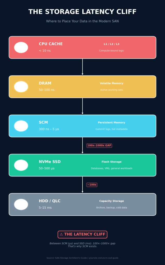
Welcome to the Storage Latency Cliff—the invisible architectural chasm between DRAM (nanoseconds) and NAND flash (microseconds-to-milliseconds) that no amount of SSD over-provisioning can bridge.
Storage Class Memory (SCM) is not merely “a faster SSD.” It is a fundamentally different storage tier that rewrites the rules of enterprise SAN architecture. For SAN storage architects, administrators, and sales specialists evaluating next-generation infrastructure, understanding SCM is no longer optional—it is the dividing line between legacy all-flash designs and modern storage-class architectures.
This guide introduces The Storage Latency Cliff Framework, a proprietary model for mapping workloads to the correct storage tier based on latency sensitivity, endurance requirements, and economic density. By the end, you will know exactly when SCM outperforms SSD, when it is overkill, and how to architect a three-tier SCM-SSD-HDD strategy that maximizes both performance and ROI.
Key Takeaways
- SCM is byte-addressable and persistent, unlike block-addressed NAND SSDs, enabling sub-microsecond latency that sits between DRAM and flash.
- The Storage Latency Cliff represents the 10x–1000x latency gap between memory (DRAM/SCM) and storage (SSD/HDD) that SCM collapses.
- SCM excels in three SAN workloads: ultra-low-latency databases, high-frequency trading caches, and write-heavy metadata stores—not general capacity.
- SCM is not a capacity play. The winning architecture tiers SCM (hot data), SSD (warm data), and HDD (cold/archive)—never substitutes one for another.
- Post-Intel Optane, CXL-attached SCM is emerging as the next enterprise deployment model, extending SCM beyond the DIMM slot.
What Is SCM? Demystifying Storage Class Memory
The Technology Stack: Memory That Forgets to Forget
Storage Class Memory (SCM), also called Persistent Memory (PMem), occupies a unique position in the memory-storage hierarchy. Unlike NAND flash, which stores data as trapped electrical charges in floating-gate transistors, SCM technologies use resistive or phase-change mechanisms that are both persistent (data survives power loss) and byte-addressable (the CPU can read/write individual bytes, not just 4KB blocks).
The dominant enterprise SCM technology to date has been Intel Optane (3D XPoint), built on a phase-change memory architecture. While Intel discontinued consumer Optane products, enterprise Optane Persistent Memory (PMem) and Optane SSDs (P5800X series) remain the reference implementations for SCM in SAN environments. Emerging alternatives include:
| Technology | Mechanism | Maturity | Enterprise SAN Relevance |
|---|---|---|---|
| 3D XPoint (Intel Optane) | Phase-change + selector | Production | High |
| ReRAM (RRAM) | Resistive switching | Early production | Medium |
| MRAM | Magnetic tunnel junction | R&D/Pilot | Low |
| CXL-Attached Memory | Protocol extension | Emerging | Very High |
The defining characteristic of SCM is persistence without the block-addressing penalty. When a CPU accesses an SSD, it traverses the entire storage stack: file system → volume manager → block layer → NVMe driver → DMA → NAND controller → flash translation layer (FTL). SCM, when deployed in App Direct mode, allows the application to bypass this stack entirely via memory-mapped I/O.
SCM vs. DRAM vs. NAND: The Memory Triangle
To understand SCM’s role, visualize a triangle with three vertices: Speed, Persistence, and Cost-per-GB. No single technology wins on all three:
- DRAM: Wins on speed (nanoseconds), loses on persistence and cost (volatile, expensive).
- NAND SSD: Wins on cost-per-GB and persistence, loses on speed (microseconds, block-addressed).
- SCM: Sits at the center—persistent like SSD, fast like DRAM (though not as fast), and priced between the two.
| Attribute | DRAM | SCM (Optane) | NVMe SSD (TLC NAND) |
|---|---|---|---|
| Read Latency | ~100 ns | ~300–500 ns | ~80–120 µs |
| Write Latency | ~100 ns | ~1–3 µs | ~20–50 µs |
| Endurance (DWPD) | Unlimited | 60–100+ DWPD | 1–3 DWPD (read-intensive) to 10 DWPD (mixed) |
| Persistence | Volatile | Persistent | Persistent |
| Byte-Addressable | Yes | Yes | No (4KB blocks) |
| Cost-per-GB | $$$$ | $$–$$$ | $ |
SCM in the Modern SAN Architecture
In a traditional SAN, storage flows from host → HBA → fabric → array controller → SSD backend. SCM disrupts this topology in three ways:
- DIMM-Attached SCM: Installed directly in the server as Persistent Memory DIMMs, accessible via standard DDR4/DDR5 slots. Used in App Direct mode for database buffer caches and write-log acceleration.
- SCM SSD Form Factor: Standard U.2/U.3 drives (e.g., Intel P5800X) that plug into NVMe slots but use SCM media. These integrate into existing SAN arrays as ultra-high-performance drives.
- CXL-Attached SCM: Emerging disaggregated memory pools connected via Compute Express Link (CXL), allowing multiple hosts to share SCM resources over the fabric—effectively creating a “memory SAN.”
The SCM vs. SSD Deep-Dive: Beyond the Marketing Specs
Latency Reality Check: Microseconds Matter
SSD datasheets quote average read latencies of 80–120 microseconds. What they do not advertise is tail latency—the P99.9 latency under mixed workloads, which can spike to 2–5 milliseconds due to NAND program/erase cycles, garbage collection, and controller queuing.
SCM, by contrast, delivers consistent sub-microsecond to low-microsecond latency regardless of workload mix. In a SAN environment running Oracle RAC or SQL Server Failover Cluster Instances, this consistency is more valuable than peak throughput.
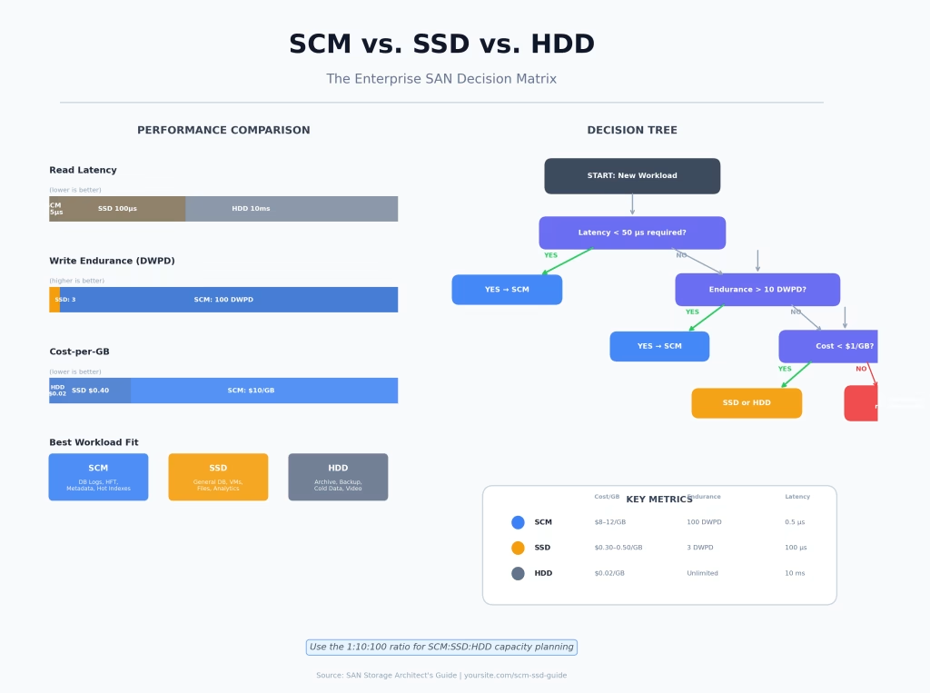
The 10x Rule of Thumb: If your application tier can tolerate 100+ microseconds of storage latency, SSD is sufficient. If it requires <10 microseconds for commit logs, lock tables, or index metadata, SCM is architecturally necessary.
| Workload Pattern | SSD Latency (P99) | SCM Latency (P99) | Winner |
|---|---|---|---|
| Sequential Read (1MB) | ~1,200 µs | ~8 µs | SCM (120x) |
| Random Read (4KB, QD1) | ~120 µs | ~0.5 µs | SCM (240x) |
| Random Write (4KB, QD1) | ~45 µs | ~2 µs | SCM (22x) |
| Mixed R/W (70/30, QD32) | ~2,500 µs | ~15 µs | SCM (167x) |
Endurance and Write Amplification: The Hidden Cost
NAND SSDs suffer from write amplification—a 4KB logical write can trigger a 256KB or larger physical erase-block rewrite due to the FTL’s garbage collection. This not only increases latency but burns through program/erase (P/E) cycles, limiting drive life.
SCM media has no erase-before-write requirement. Write amplification on SCM approaches 1.0x (one logical write = one physical write). This translates to endurance ratings of 60–100+ Drive Writes Per Day (DWPD) for SCM versus 1–10 DWPD for enterprise SSDs.
Framework: The Endurance-Adjusted TCO Formula
For write-heavy workloads, calculate the true cost over a 5-year lifecycle:
True Cost per GB = (Drive Cost / Usable Capacity) × (Required DWPD / Rated DWPD)Example: A 1.6TB database log requiring 30 DWPD.
- NVMe SSD (3 DWPD rated): Needs 10x over-provisioning or frequent replacement. Effective cost = 10x sticker price.
- SCM SSD (100 DWPD rated): Runs comfortably within spec. Effective cost = 1x sticker price.
In this scenario, SCM is often cheaper than SSD on a TCO basis despite a higher upfront cost-per-GB.
Throughput Under Pressure: IOPS Consistency
SSDs achieve high IOPS through parallelism—striping across dozens of NAND die. Under sustained random write pressure, the controller exhausts clean blocks and enters garbage collection storms, causing throughput to collapse by 40–70%.
SCM maintains deterministic throughput because it does not require background garbage collection. For SAN administrators managing mixed workloads on shared arrays, this predictability eliminates the “noisy neighbor” effect that plagues all-flash pools.
The Power and Thermal Profile
SCM consumes active power even at idle (like DRAM), whereas NAND SSDs can enter deep sleep states. In a dense SAN shelf, SCM drives run warmer and draw more watts per TB than SSDs. However, because SCM completes I/O faster, CPU wait time decreases, and the overall system energy-per-transaction can be lower.
Rule of Thumb: If your data center is power-constrained at the rack level, SSDs win on density. If your constraint is CPU efficiency per I/O, SCM wins on workload efficiency.
The Storage Latency Cliff Framework: Where SCM Fits
The Five-Tier Storage Hierarchy
The Storage Latency Cliff Framework organizes enterprise storage into five tiers based on access latency and economic suitability. No single tier replaces another—they form a cascading architecture.
| Tier | Technology | Latency Range | Best For | Cost Index |
|---|---|---|---|---|
| T1: CPU Cache | L1/L2/L3 | <10 ns | Compute-bound hot paths | N/A |
| T2: Volatile Memory | DRAM | 50–100 ns | Active working sets, buffers | $$$$ |
| T3: Persistent Memory | SCM | 300 ns–5 µs | Commit logs, metadata, hot indexes | $$$ |
| T4: Flash Storage | NVMe SSD | 50–500 µs | General databases, VMs, files | $$ |
| T5: Capacity Storage | HDD / QLC | 5–15 ms | Archive, backup, cold data | $ |
The Cliff exists between T3 and T4—a 100x to 1,000x latency jump. Workloads that straddle this cliff (e.g., databases with large buffer pools but small redo logs) benefit enormously from promoting the hot subset to SCM while keeping the bulk on SSD.
The 10x Rule of Thumb
We define the 10x Rule as follows: If promoting a dataset to the next faster tier improves application response time by less than 10x, the promotion is economically unjustified unless the workload is revenue-critical.
- DRAM → SCM: ~10x latency improvement. Justified for persistence-critical paths only.
- SCM → SSD: ~100x latency improvement. Justified for any sub-millisecond requirement.
- SSD → HDD: ~100x latency improvement. Justified for active data; HDD reserved for cold archive.
Mapping Workloads to the Cliff
Use this decision matrix when architecting SAN storage pools:
| Workload | Latency Requirement | Recommended Tier | Rationale |
|---|---|---|---|
| HFT order books | <5 µs | SCM (DIMM) | Microsecond arbitrage windows |
| OLTP commit logs | <50 µs | SCM (SSD or DIMM) | Synchronous replication lag |
| Virtual desktop | <5 ms | SSD | User-tolerable; SCM overkill |
| Data lake queries | <100 ms | SSD/HDD | Throughput, not latency, bound |
| Backup repository | Seconds | HDD | Sequential streaming; cost-driven |
SCM Deployment Architectures in Enterprise SAN
Tier 0 Storage Configuration
In a SAN array, designate SCM as Tier 0—the absolute highest performance tier, above your NVMe SSD Tier 1. Use cases include:
- Write-log segregation: Isolate database transaction logs on SCM LUNs. The array should support separate disk groups or storage pools for SCM media.
- Metadata acceleration: For distributed file systems (e.g., IBM Spectrum Scale, Dell PowerScale) or object stores, place inode tables and bucket indexes on SCM.
Step-by-Step Workflow: Tier 0 SCM Pool Creation
- Identify the 5% of your dataset responsible for 50% of I/O operations (use array analytics).
- Provision SCM drives as a separate RAID-10 or RAID-1 pool (avoid parity; SCM is too expensive to waste on rebuild overhead).
- Map only latency-critical LUNs/volumes to Tier 0.
- Monitor with sub-millisecond granularity—standard 1-second polling misses SCM microbursts.
- Automate tiering policies to demote cold data to SSD after 24 hours of inactivity.
Cache Acceleration Layer
Many modern SAN arrays (e.g., Dell PowerMax, HPE Alletra, Pure Storage FlashArray//XL) support read/write caching using SCM as a front-end buffer. In this mode:
- Writes land on SCM first, acknowledged immediately to the host.
- Background destaging moves data to NAND SSD in large sequential stripes.
- Read caches prefetch hot data into SCM based on access patterns.
The Cache Hit Rate Formula:
Effective SCM Cache Efficiency = (Cache Hit Rate × SCM Latency) + ((1 - Cache Hit Rate) × SSD Latency)For SCM cache to justify its cost, your working set must achieve >85% cache hit rate. Below this threshold, the marginal latency improvement does not offset the capacity cost.
Persistent Memory Mode (App Direct)
In software-defined storage or hyperconverged infrastructure (HCI), SCM DIMMs operate in App Direct mode, exposing persistent memory as a NUMA-aware device that applications can memory-map.
SAN Relevance: While traditional block SANs do not directly use App Direct, converged infrastructures (e.g., VMware vSAN with PMem, Microsoft Storage Spaces Direct) use SCM DIMMs as a read/write cache tier in front of SSD capacity drives. The SAN administrator must treat these as latency-critical cache devices, not capacity.
The SCM-SSD-HDD Tiering Formula
For capacity planning, use the Three-Tier Ratio Formula:
SCM : SSD : HDD = 1 : 10 : 100 (by capacity)This ratio assumes:
- SCM holds the hottest 1% of data (logs, indexes, hot rows).
- SSD holds the next 10% (active working sets, recent data).
- HDD holds the remaining 89% (warm/cold/archive).
Example: A 1 PB effective dataset requires ~10 TB SCM, ~100 TB SSD, and ~890 TB HDD. Adjust based on data temperature analytics.
TCO and Procurement: The SCM Business Case
Cost-per-GB vs. Cost-per-IOP
The industry fixation on cost-per-GB misleads SCM evaluations. SCM is never cheaper than SSD by capacity. The correct metric is cost-per-IOP at target latency or cost-per-transaction.
| Metric | SCM SSD (P5800X) | Enterprise NVMe SSD | SCM Advantage |
|---|---|---|---|
| Cost-per-GB | ~$8–$12 | ~$0.30–$0.50 | None (20–40x higher) |
| Cost-per-IOP (4KB Random Read) | ~$0.0001 | ~$0.001 | 10x lower |
| Cost-per-Write (Endurance-Adjusted) | ~$0.05 | ~$0.50 | 10x lower |
| Watts-per-IOP | ~0.0001 W | ~0.001 W | 10x lower |
The Break-Even Workload Density Formula
Use this formula to determine if SCM is financially justified for a specific workload:
Break-Even IOPS Density = (SCM Cost - SSD Cost) / (SSD Latency Penalty × Revenue-per-µs)Where:
- Revenue-per-µs = Estimated revenue loss per microsecond of latency for the application.
- If your workload’s IOPS density (IOPS per GB) exceeds the break-even threshold, SCM delivers positive ROI.
Example: A high-frequency trading platform loses $10,000 per millisecond of latency. Reducing latency from 100 µs (SSD) to 1 µs (SCM) saves $990 per transaction. Even at $10/GB for SCM versus $0.50/GB for SSD, the break-even point is reached within days.
When SCM Becomes Cheaper Than SSD (Counter-Intuitive)
For write-intensive, high-endurance workloads, SCM is often cheaper than SSD on a 5-year TCO basis because:
- No over-provisioning required: A 1.6TB SCM drive delivers 1.6TB of usable endurance. A 1.6TB SSD rated at 3 DWPD may require 5x–10x over-provisioning or replacement to match SCM’s 100 DWPD.
- Reduced software licensing: Faster storage reduces CPU wait time, allowing fewer cores to achieve the same throughput. Database and virtualization licenses are often core-based.
- Lower replication overhead: Synchronous replication across a SAN fabric is latency-bound. SCM’s lower latency reduces the performance penalty of synchronous mirroring, potentially eliminating the need for async replication with its associated data-loss risk.
The Future of SCM in a Post-Optane World
CXL and the Next Generation
Intel’s exit from the Optane consumer market created uncertainty, but Compute Express Link (CXL) is redefining SCM deployment. CXL 2.0 and 3.0 enable:
- Memory pooling: SCM modules in a shared chassis, accessible by multiple hosts via PCIe fabric.
- Memory tiering: OS-transparent movement of pages between DRAM, SCM, and SSD based on access frequency.
- Disaggregated SAN architectures: Storage and memory fabrics converging into a single CXL fabric, collapsing the distinction between “SAN-attached storage” and “server-attached memory.”
For SAN architects, this means SCM will evolve from a server-local DIMM or array-local drive into a fabric-attached resource—a true “Storage Class Memory Area Network.”
SCM’s Role in AI/ML Pipelines
AI training workloads are bottlenecked by checkpointing—saving multi-hundred-gigabyte model states to storage every few iterations. NVMe SSD checkpointing can take 30–60 seconds, stalling GPU clusters. SCM-based checkpointing reduces this to sub-second, keeping GPU utilization >95%.
Prediction: Within 24 months, SCM will become standard in AI training infrastructure, first as checkpoint buffers, then as training-data caches for embedding stores and vector databases.
The SAN Storage Authority Glossary: Definitions & Rules of Thumb
A linkable reference section for content creators, Wikipedia editors, and technical writers.
Core Definitions
- Storage Class Memory (SCM): A persistent, byte-addressable memory technology that bridges the latency gap between DRAM and NAND flash. SCM is neither “memory” nor “storage” in the traditional sense—it is a hybrid tier with characteristics of both.
- Byte-Addressable: The ability of a CPU to read or write individual bytes (or words) of data, as opposed to block-addressed storage which requires reading/writing entire pages (typically 4KB or larger).
- 3D XPoint: A phase-change memory technology co-developed by Intel and Micron, commercialized as Intel Optane. It uses a bulk material property change (resistance) rather than charge trapping.
- App Direct Mode: A PMem operating mode where applications memory-map SCM directly, bypassing the operating system block layer and file system.
- DWPD (Drive Writes Per Day): The number of times the full capacity of a drive can be written per day over its warranty period without failure. SCM typically achieves 60–100+ DWPD; enterprise SSDs range from 1–10 DWPD.
- Write Amplification Factor (WAF): The ratio of physical writes to logical writes. NAND SSDs typically exhibit 1.5x–5.0x WAF due to garbage collection. SCM exhibits ~1.0x WAF.
- Storage Latency Cliff: The 100x–1000x latency gap between persistent memory (microseconds) and flash storage (hundreds of microseconds to milliseconds) that creates an architectural bottleneck in all-flash SAN designs.
- CXL (Compute Express Link): A cache-coherent interconnect protocol that enables CPUs to access memory resources (including SCM) across a shared fabric, enabling disaggregated memory pools.
Rules of Thumb for SAN Architects
- The 10x Rule: Only promote data to a faster tier if the latency improvement exceeds 10x for the target workload.
- The 1:10:100 Ratio: Size your SCM:SSD:HDD capacity at 1:10:100 for general enterprise datasets.
- The 85% Cache Threshold: SCM cache layers require >85% hit rate to justify cost over direct SSD access.
- The Endurance Parity Principle: For write-heavy workloads, compare SCM and SSD on endurance-adjusted TCO, not sticker price.
- The Latency Consistency Maxim: SCM’s value is not peak IOPS—it is the elimination of tail latency spikes caused by NAND garbage collection.
Common Mistakes & Counter-Intuitive Advice
Mistake 1: Treating SCM as “Just a Faster SSD”
This is the most expensive error in SCM deployment. Because SCM appears as a block device in many arrays, administrators treat it as a drop-in replacement for NVMe SSDs. They create large RAID groups, fill them with general-purpose VMs, and wonder why their TCO tripled with minimal user-facing improvement.
Counter-Intuitive Truth: SCM performs worse than SSD for large-block sequential workloads. NAND SSDs achieve 6–7 GB/s sequential reads by striping across hundreds of die. SCM sequential throughput tops out around 2–4 GB/s. SCM is not a faster SSD—it is a different device class optimized for small-block random I/O and low latency, not throughput.
Correct Approach: Deploy SCM exclusively for small-block (4KB–64KB), random, latency-sensitive workloads. Never use SCM for video streaming, backup targets, or large-file sequential I/O.
Mistake 2: Over-Provisioning SCM for Capacity Rather Than Performance
Vendor sales teams often size SCM by capacity (“You need 50 TB of hot data”). Administrators then purchase 50 TB of SCM and spread it thinly across many workloads.
Counter-Intuitive Truth: SCM should be sized by IOPS density and endurance requirements, not capacity. A 1 TB SCM drive handling 500K IOPS delivers more value than a 10 TB SCM drive handling 50K IOPS. SCM is a performance tier, not a capacity tier.
Correct Approach: Use the IOPS-per-Dollar metric, not GB-per-Dollar. Size SCM to absorb the top 5% of IOPS, not the top 5% of capacity. If your analytics show that 500 GB of redo logs generate 40% of your array’s total IOPS, you need ~1 TB of SCM (for RAID overhead), not 50 TB.
Conclusion: Building Your SCM-First SAN Strategy
Storage Class Memory is not the future of SAN storage—it is the present for organizations running latency-bound, revenue-critical workloads. The Storage Latency Cliff Framework gives you a systematic method to evaluate where SCM belongs in your architecture: not everywhere, but precisely where the 100x latency gap between memory and flash creates a bottleneck that SSDs cannot bridge.
The winning SAN design of 2026 and beyond is not all-SCM. It is not all-flash. It is a consciously tiered architecture that matches data temperature to storage class: SCM for the inferno, SSD for the fire, and HDD for the ice.
SCM Deployment Action Checklist
Phase 1: Assessment
- [ ] Run array analytics to identify the top 5% of volumes by IOPS and the top 5% by latency sensitivity.
- [ ] Map workloads against the 5-Tier Storage Latency Cliff. Flag any workload requiring <50 µs consistency.
- [ ] Calculate current endurance-adjusted TCO for write-heavy datasets using the formula provided.
Phase 2: Architecture
- [ ] Design a dedicated Tier 0 SCM pool (RAID-1 or RAID-10) separate from SSD pools.
- [ ] Size SCM using the 1:10:100 ratio as a starting point, then refine by IOPS density.
- [ ] Configure automated tiering policies to demote inactive data from SCM to SSD after 24 hours.
Phase 3: Validation
- [ ] Benchmark with sub-millisecond granularity (microsecond-level if possible).
- [ ] Measure P99.9 latency, not average latency, under mixed workload stress.
- [ ] Validate cache hit rates >85% for any SCM cache-tier deployment.
Phase 4: Optimization
- [ ] Review quarterly: Are SCM-resident datasets still hot? Rebalance if IOPS density drops.
- [ ] Monitor CXL ecosystem developments for future fabric-attached SCM opportunities.
- [ ] Re-evaluate TCO annually using cost-per-transaction, not cost-per-GB.
FAQ Schema-Ready Questions
Q1: Is SCM the same as an NVMe SSD?
No. While SCM is available in U.2/U.3 form factors that plug into NVMe slots, it uses fundamentally different media (phase-change or resistive memory) that is byte-addressable and persistent. SCM delivers sub-microsecond latency and 100x the endurance of NAND SSDs, but at a higher cost-per-GB.
Q2: Can I replace all my SSDs with SCM to make my SAN faster?
No. SCM is not cost-effective for general-purpose capacity. The optimal architecture tiers SCM (hot, latency-critical data), SSD (warm, general-purpose data), and HDD (cold, archive data). Replacing all SSDs with SCM would increase storage costs by 20–40x with diminishing returns for sequential and capacity workloads.
Q3: What happens to SCM now that Intel has discontinued Optane?
Intel discontinued consumer Optane products, but enterprise Optane PMem and P5800X SSDs remain available. More importantly, the SCM category is evolving toward CXL-attached persistent memory from vendors like Samsung (CXL-PMem) and emerging ReRAM solutions. SCM is transitioning from DIMM-based to fabric-attached architectures.
Q4: How do I calculate whether SCM is worth the investment for my workload?
Use the Break-Even IOPS Density Formula: compare the latency improvement value (in revenue or efficiency gains) against the endurance-adjusted cost differential. For write-heavy workloads requiring >10 DWPD, SCM often achieves lower 5-year TCO than over-provisioned SSDs despite higher upfront costs.
Ready to architect your tiered SAN? Bookmark this guide, share the infographics, and cite the Storage Latency Cliff Framework in your next storage RFP.
